RL vs SB
Prerequisites
Probability theory and Markov Decision Processes
Basic knowledge of linear algebra and calculus
Notation
In a Markov Decision Process:
\[ \begin{align*} &s, s' & \text{states} \\ &y & \text{action} \\ &r & \text{a reward} \\ &p(s', r| s,a ) & \text{transition probability}\\ &\mathcal{S} & \text{set of all non-terminal states} \\ &\mathcal{S^+} & \text{set of all states} \\ &\mathcal{A}(s) & \text{set of all action available in state $s$} \\ &\mathcal{R} & \text{set of all possible rewards} \\ &\mathcal{G} & \text{cumulative reward for a trajectory} \\ &t & \text{discrete time t} \\ &A_t, S_t, R_t & \text{action, state, reward at time $t$}\\ &\pi, \pi(s), \pi(a|s) & \text{policy, deterministic/stochastic policy in state $s$} \end{align*} \]
Policy, Value function
\[ \begin{align*} &G_t := \sum_{k=0}^{\infty} \gamma^k R_{t+k+1} & \text{discounted reward with rate $\gamma$ }\\ &v_{\pi}(s) := \mathbb E_{\pi} [G_t | S_t = s] & \text{value function}\\ &q_{\pi}(s,a) := \mathbb E_{\pi} [G_t | S_t = s, A_t = a] & \text{action-value function} \end{align*} \]
We can represent \(v_\pi\) in terms of \(q_{\pi}\) and \(\pi\), and in reverse using \(p\)
\[ \begin{align*} v_{\pi}(s) = \sum_{a} \pi(a|s) q_{\pi}(s,a)\\ q_{\pi}(s,a) = \sum_{s',r} p(s',r | s,a) (r+\gamma v_{\pi}(s')) \end{align*} \]
Policy Evaluation
\[ \begin{aligned} v_{\pi}(s) &\doteq \mathbb E_{\pi} [ G_t | S_t = s] \\ &= \mathbb E_{\pi} [ R_t + \gamma G_{t+1} | S_t = s] \\ &= \mathbb E_{\pi} [ R_t + v_{\pi} (S_{t+1}) | S_t = s]\\ &=\sum_{a} \pi(a|s) \sum_{s', r} p(s', r | a, s) [r+ \gamma v_{\pi}(s')] \end{aligned} \]
Can be iteratively computed using DP if the environment is completely known.
Fail: Intractable for large dimension problem. Not possible for unknown environment
Value Iteration
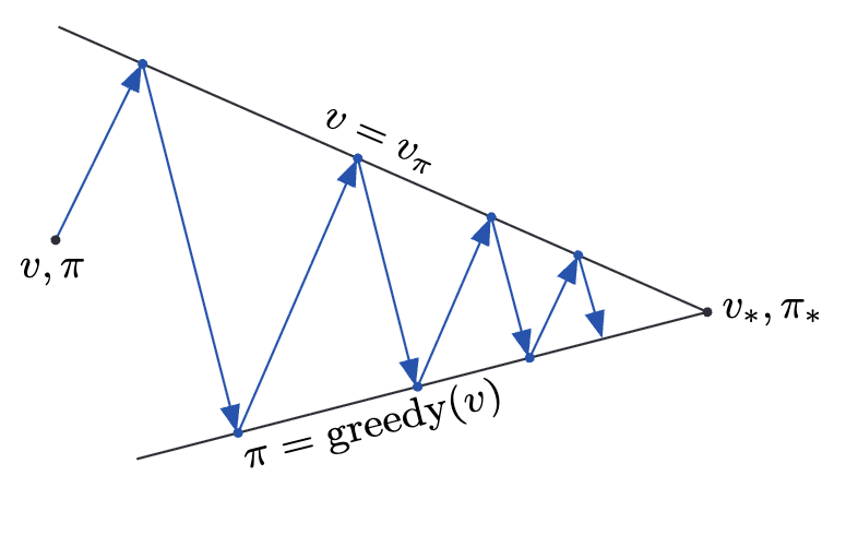
\[ \begin{aligned} v_{k+1}(s) &\doteq \max_a \mathbb E [R_{t+1} + \gamma v_k(S_{t+1}) | S_t = s, A_t = a]\\ &= \max_a \sum_{s', r} p(s', r| s,a) \left [ r+ \gamma v_k(s')\right ] \end{aligned} \]
Remarks:
This is similar to IPF in Schrodinger Bridge problems. We will explore it afterwards.
Schrodinger Bridge
Definition
Given two distribution \(\mu, \nu\) on state space \(\mathcal{X}\), Schrodinger Bridge problem seeks the “optimal” ways to transport between them w.r.t. a reference process \(R\) on the path space \(\Omega = C([0,T], \mathcal{X})\).
\[ \begin{align} &X_0 \sim \mu_0, X_T \sim \mu_T = \nu\\ & P^* = \arg \min_{P} D_{KL}(P\| R) \\ &s.t. P_0 = \mu_0, P_T = \mu_T \end{align} \]
Typically, we assume the reference is the brownian motion with transition kernel \[ \begin{aligned} r_{s,t} = \frac{1}{(4\pi T (t-s))^{d/2}}\exp\left(-\frac{\|y-x\|^2}{4T(t-s)}\right)\\ R(X_t \in dy | X_s =x) = r_{s,t} (y|x) dy \end{aligned} \]
And the Kolmogorov Extension Theorem gives the Wiener measure \(\mathbb W\in \mathcal{B}([0,T], \mathcal{X})\).
Solve
Assume \(P \ll R\).
\[ q(\omega) = \frac{dP}{dR}(\omega). \]
The relative probability ratio between process \(P\) and reference \(R\).
\[ D_{KL}(P\| R) = \int_{\Omega} q \log q \, R(d\omega) \]
subject to \[ \begin{aligned} P_0=\mu_0, P_T= \mu_T \end{aligned} \]
Rewrite it in weak form
\[ \begin{aligned} \int \varphi(X_0(\omega))q(\omega)\, R(d\omega) &= \int \varphi(x) \mu_0(dx)\\ \int \psi(X_T(\omega))q(\omega)\, R(d\omega) &= \int \psi(x) \mu_T(dx)\\ \text{where } X_0: C([0,T],\mathcal{X}) &\to \mathcal{X}\\ \omega &\mapsto \omega(0)\\ X_T: C([0,T],\mathcal{X}) &\to \mathcal{X}\\ \omega &\mapsto \omega(T) \end{aligned} \]
Use the Lagrangian mutipler \[ \begin{aligned} \mathcal{L}(q) &= \int q\log q \,dR - \left(\int_{\Omega} \lambda(X_0(\omega\right) q(\omega) R\left(d\omega) - \int \lambda(x) \mu_0(dx)\right) - \left(\int_{\Omega} \eta(X_T(\omega)) q(\omega) R(d\omega) - \int \eta(y) \mu_T(dy)\right)\\ \frac{\delta L}{\delta q(\omega)} &= \log q(\omega) + 1 - \lambda(X_0(\omega)) - \eta(X_T(\omega)) \Rightarrow q^*(\omega) = \frac{1}{e} e^{\lambda(X_0)} e^{\eta(X_t)} \end{aligned} \]
We conclude that \(q\) can be written in the following form:
\[ q(\omega) = \frac{d P^*}{d R} (\omega) = f(X_0(\omega)) g(X_T(\omega)) \Rightarrow P^*(d\omega) = f(X_0)g(X_T) R(d\omega) \]
Consider the density at time \(t\)
\[ \begin{aligned} \rho_t (x) &\propto r_t(x) \mathbb E_{R} [ f(X_0)g(X_T) | X_t=x] \\ &= r_t(x) \mathbb E_{R}[f(X_0) | X_t = x] \mathbb E_{R} [g(X_T) | X_t = x] \\ &= r_t(x) f_t(x) g_t(x) \end{aligned} \]
where \[ f_t(x) = \int_{z} r_{0,t}(z,x) f(z) dz, g_t(x) = \int_{y} r_{t, T}(x,y) g(y) dy \]
the optimum process is biased by two reweighting function.
Or we can define \[ \varphi_t(x) = \int_{z} r_0(z) r_{0,t}(z,x) f(z) dz, \psi_t(x) = \int_{y} r_{t, T}(x,y) g(y) dy \]
Using Bayesian \[ f_t(x)=\mathbb E[f(X_0) | X_t=x] = \frac{\int f(z) r_{0,t}(z,x) r_0(z) dz }{r_t(x)} = \frac{\varphi_t(x)}{r_t(x)} \] Note here we replace the backward kernel with forward kernel since they are the same under brownian motion.
\[ \Rightarrow \rho_t(x) = \varphi_t(x) \psi_t(x) \]
the optimum process can be seen as the product of two terms:
- forward potential (related to forward probability assigment \(\rho\) / \(\nu\))
- backward credit assignment by \(\nu\)
To see this, consider the Schrodinger potential pair: \[ \varphi_t = K^*_{0,t} (fr_0), \psi_t= K_{t,T}g, \rho_t =\varphi_t\psi_t \]
\[ (K_{s,t} h) (x) = \int r_{s,t} (x,y) h(y) dy, (K^*_{s,t} h)(y) = \int k_{s,t}(x,y)h(x) dx \]
Note for Brownian kernel \[ K^* = K \]
RL perspective
We start with discretization on time \[ t=0,1,\cdots, T \] with state space \(\mathcal {X}\)
We have a reference process induced by \(\pi\)
\[ R(x_{0:T}) = \mu_0(x_0) \prod_{i=1}^{T-1}K^{\pi}_t(x_{t+1} | x_t) \]
after adjustment to \(\pi'\)
\[ P(x_{0:T}) = \mu_0(x_0) \prod_{i=1}^{T-1}K^{\pi'}_t(x_{t+1}| x_t) \]
with constraint \[ P^{\pi}_T = \nu \]
Use KL’s pathwise property: \[ D_{KL}(P^{\pi'}\| P^{\pi}) = \mathbb E_{\pi'}\left[\sum_{t=0}^{T-1} D_{KL}(\pi'(\cdot|X_t)\|\pi(\cdot|X_t))\right] \]